Gates of Olympus RTP Analysis: Results From 40,000 Spins
See what 40,000 demo spins reveal about Gates of Olympus RTP, Ante Bet bonus frequency, dry spells, multipliers, and statistical uncertainty.

Can a Gates of Olympus RTP analysis based on 40,000 demo spins tell us whether the advertised RTP and Ante Bet mechanics behave as expected?
This study uses Python, probability, and statistical inference to compare 20,000 Regular paid spins with 20,000 Ante paid spins. It focuses on four practical questions:
- How often did each mode trigger the free-spins bonus?
- Was the observed Ante increase compatible with the advertised
2×chance? - How unstable was the observed RTP over this sample size?
- Did multiplier frequency or multiplier size differ between modes?
The dataset provides useful evidence about this collected sample, but it is not a regulatory audit, an RNG certification, or proof that every real-money version uses the same configuration.
Responsible-gambling note: RTP is a long-run mathematical expectation, not a promise for a player or session. A temporary return above 100% does not turn a negative-expectation game into a profitable strategy.
Gates of Olympus RTP Analysis: Key Findings
The raw file contains 42,315 recorded events. After separating 2,315 free-spin rows from the paid wagers, the analysis contains exactly 40,000 paid spins across 40 sessions.
| Metric | Regular mode | Ante mode |
|---|---|---|
| Paid spins | 20,000 | 20,000 |
| Bonus triggers | 39 | 112 |
| Observed bonus-trigger rate | 0.195% | 0.560% |
| Approximate mean spins per bonus | 513 | 179 |
| Observed RTP | 89.263% | 101.797% |
| 95% row-bootstrap RTP interval | 78.52%–101.23% | 87.61%–117.85% |
| Winning base spins with a multiplier | 295 | 346 |
| Multiplier-event rate | 1.475% | 1.730% |
The observed bonus-rate ratio was:
0.560% / 0.195% = 2.872×A large-sample 95% confidence interval for that rate ratio was approximately:
1.996× to 4.132×The sample strongly rejects equal bonus rates. However, a direct test against an exact 2× rate ratio produced p = 0.0513, so the data are narrowly compatible with the advertised doubling claim at the conventional 5% significance level.
The RTP estimates are much less precise. Both bootstrap intervals are wide and contain the publicly listed 96.50% RTP, so this sample does not provide strong evidence that either mode’s long-run RTP differs from that value.
Table of Contents
- Game rules and study scope
- How the dataset was normalized
- Ante Bet bonus frequency
- Bonus dry-spell risk
- Observed RTP and confidence intervals
- Multiplier analysis
- Limitations
- Frequently asked questions
Gates of Olympus Rules and Study Scope
Pragmatic Play’s public Gates of Olympus page describes the standard game as follows:
- a 6×5 layout with tumbling reels;
- wins from 8–30 matching symbols anywhere on the screen;
- multiplier symbols with values up to
500×; - 15 free spins when four or more scatter symbols land;
- a listed RTP of
96.50%.
The official public description is available on the Pragmatic Play Gates of Olympus page.
The demo build used during collection also displayed an Ante option that:
- raised the stake from
0.20to0.25, a 25% increase; - advertised double the chance of triggering the free-spins feature.
Game features, available RTP configurations, and regional options can vary by build or market. A fully reproducible project should therefore archive the exact help-screen rules and RTP shown in the tested version.
What this study can evaluate
The data can be used to estimate:
- observed bonus frequency;
- uncertainty around the Ante-to-Regular rate ratio;
- waiting-time risk under an independent-spin model;
- sample RTP and bootstrap uncertainty;
- multiplier-event frequency and conditional multiplier values.
What this study cannot prove
The data cannot establish:
- how the internal RNG is implemented;
- whether demo and real-money deployments are identical;
- whether every operator uses the same RTP configuration;
- whether the theoretical probability table is correct;
- whether the game satisfies a particular regulatory standard.
For those reasons, this is an observational statistical analysis, not a certified audit.
How the 40,000-Spin Dataset Was Normalized
The raw dataset contains these columns:
| Column | Meaning |
|---|---|
round_id | Round identifier recorded by the collector |
bet | Amount wagered on that event |
win | Return or cumulative bonus return recorded at that event |
multiplier | Multiplier value recorded by the collector |
is_ante | Whether Ante mode was active |
is_bonus | Whether the row belonged to a free-spin sequence |
The file contains:
40,000 paid-spin rows
+ 2,315 free-spin rows
= 42,315 recorded events
There are 20 Regular sessions and 20 Ante sessions, each containing 1,000 paid spins.
Why one paid round is the correct unit
RTP must be calculated from paid rounds, not from individual free spins.
A paid round consists of:
one wager
+ its base-game return
+ any bonus return caused by that wager
Treating every free-spin row as a separate wager would inflate the number of observations and distort RTP.
The bonus rows are cumulative
The dataset contains 151 bonus sequences:
- 39 triggered in Regular mode;
- 112 triggered in Ante mode;
- 141 sequences contained 15 free spins;
- 10 sequences contained 20 rows because of retriggers.
Within every sequence, the win field is non-decreasing. This indicates that the free-spin rows store a cumulative bonus total, not an independent win for each row.
The correct normalization rule for this file is therefore:
- keep every non-bonus row as one paid round;
- identify each consecutive bonus sequence;
- attach only the final cumulative bonus value to the paid row immediately before that sequence;
- mark that paid round as a bonus trigger.
Summing every bonus row would massively overstate returns.
Reproducible Python normalization
from __future__ import annotations

import numpy as np
import pandas as pd

raw = pd.read_csv("spins-dataset.csv")

# A new session starts when round IDs reset or the mode changes.
session_start = (
    raw["round_id"].le(raw["round_id"].shift())
    | raw["is_ante"].ne(raw["is_ante"].shift())
)
session_start.iloc[0] = True

raw["session_id"] = (
    session_start.cumsum().map(lambda value: f"s{value:03d}")
)

# Start with one row for every paid spin.
rounds = (
    raw.loc[~raw["is_bonus"]]
    .copy()
    .reset_index(names="source_index")
)

rounds["paid_round_id"] = np.arange(1, len(rounds) + 1)
rounds["mode"] = np.where(
    rounds["is_ante"],
    "Ante",
    "Regular",
)
rounds["wager"] = rounds["bet"]
rounds["total_return"] = rounds["win"]
rounds["bonus_triggered"] = False
rounds["base_multiplier"] = rounds["multiplier"]

bonus_mask = raw["is_bonus"].to_numpy()

bonus_starts = np.flatnonzero(
    bonus_mask & np.r_[True, ~bonus_mask[:-1]]
)
bonus_ends = np.flatnonzero(
    bonus_mask & np.r_[~bonus_mask[1:], True]
)

source_to_paid_index = {
    int(source_index): paid_index
    for paid_index, source_index
    in enumerate(rounds["source_index"])
}

for start, end in zip(bonus_starts, bonus_ends):
    trigger_source_index = start - 1
    paid_index = source_to_paid_index[trigger_source_index]

    cumulative_bonus_return = raw.iloc[end]["win"]

    rounds.loc[paid_index, "bonus_triggered"] = True
    rounds.loc[paid_index, "total_return"] += (
        cumulative_bonus_return
    )
Validate the normalized paid-round table
REQUIRED_COLUMNS = {
    "paid_round_id",
    "session_id",
    "mode",
    "wager",
    "total_return",
    "bonus_triggered",
    "base_multiplier",
}


def validate_rounds(rounds: pd.DataFrame) -> None:
    missing = REQUIRED_COLUMNS.difference(rounds.columns)
    if missing:
        raise ValueError(
            f"Missing required columns: {sorted(missing)}"
        )

    if len(rounds) != 40_000:
        raise ValueError("Expected exactly 40,000 paid rounds.")

    if rounds["paid_round_id"].duplicated().any():
        raise ValueError(
            "Each paid_round_id must appear exactly once."
        )

    if not rounds["mode"].isin(["Regular", "Ante"]).all():
        raise ValueError(
            "mode must contain only Regular or Ante."
        )

    if (rounds["wager"] <= 0).any():
        raise ValueError(
            "Every paid round must have a positive wager."
        )

    if (rounds["total_return"] < 0).any():
        raise ValueError("Returns cannot be negative.")

    mode_counts = rounds["mode"].value_counts()
    if mode_counts.to_dict() != {
        "Regular": 20_000,
        "Ante": 20_000,
    }:
        raise ValueError(
            "Expected 20,000 paid rounds in each mode."
        )


validate_rounds(rounds)
Why the actual Ante wager matters
The raw file records:
Regular wager: 0.20
Ante wager:    0.25
The RTP denominator must use the actual amount paid. Using 0.20 for an Ante spin that cost 0.25 would overstate Ante RTP by 25%.
For this dataset, the correct field is already present:
rounds["wager"] = rounds["bet"]Does Ante Bet Increase Gates of Olympus Bonus Frequency?
Define:
p_R = probability of a bonus trigger in Regular mode
p_A = probability of a bonus trigger in Ante mode
The observed bonus rates were:
Regular: 39 / 20,000  = 0.195%
Ante:   112 / 20,000  = 0.560%
The observed rate ratio was:
RR = p_A / p_R = 2.8718Calculate the bonus rates
def bonus_summary(rounds: pd.DataFrame) -> pd.DataFrame:
    result = (
        rounds.groupby("mode", observed=True)
        .agg(
            paid_rounds=("paid_round_id", "size"),
            bonus_hits=("bonus_triggered", "sum"),
        )
    )

    result["hit_rate"] = (
        result["bonus_hits"] / result["paid_rounds"]
    )
    result["hit_rate_percent"] = result["hit_rate"] * 100
    result["mean_wait_spins"] = 1 / result["hit_rate"]

    return result


bonus_stats = bonus_summary(rounds)
print(bonus_stats)
Test whether the two rates are equal
Because bonus triggers are rare, Fisher’s exact test is a useful primary comparison.
import numpy as np
from scipy.stats import fisher_exact

regular = rounds[rounds["mode"].eq("Regular")]
ante = rounds[rounds["mode"].eq("Ante")]

regular_hits = int(regular["bonus_triggered"].sum())
ante_hits = int(ante["bonus_triggered"].sum())

observed = np.array([
    [ante_hits, len(ante) - ante_hits],
    [regular_hits, len(regular) - regular_hits],
])

odds_ratio, p_equal_rates = fisher_exact(
    observed,
    alternative="two-sided",
)

print(f"Fisher odds ratio: {odds_ratio:.4f}")
print(f"P-value: {p_equal_rates:.12g}")
The exact-test p-value is approximately:
2.12 × 10^-9This is extremely strong evidence against equal bonus-trigger probabilities in the two modes.
Test the advertised 2× claim directly
Rejecting equal rates does not test whether the true ratio equals 2.
The relevant hypothesis is:
H0: p_A / p_R = 2A log-rate-ratio approximation gives:
from dataclasses import dataclass
from math import exp, log, sqrt

from scipy.stats import norm


@dataclass(frozen=True)
class RateRatioResult:
    estimate: float
    ci_low: float
    ci_high: float
    z_statistic: float
    p_value: float


def rate_ratio_test(
    ante_hits: int,
    ante_total: int,
    regular_hits: int,
    regular_total: int,
    null_ratio: float = 2.0,
    alpha: float = 0.05,
) -> RateRatioResult:
    if ante_hits <= 0 or regular_hits <= 0:
        raise ValueError(
            "This approximation requires non-zero hit counts."
        )

    ante_rate = ante_hits / ante_total
    regular_rate = regular_hits / regular_total
    ratio = ante_rate / regular_rate

    se_log_ratio = sqrt(
        (1 / ante_hits)
        - (1 / ante_total)
        + (1 / regular_hits)
        - (1 / regular_total)
    )

    critical = norm.ppf(1 - alpha / 2)

    ci_low = exp(log(ratio) - critical * se_log_ratio)
    ci_high = exp(log(ratio) + critical * se_log_ratio)

    z_statistic = (
        log(ratio) - log(null_ratio)
    ) / se_log_ratio

    p_value = 2 * norm.sf(abs(z_statistic))

    return RateRatioResult(
        estimate=ratio,
        ci_low=ci_low,
        ci_high=ci_high,
        z_statistic=z_statistic,
        p_value=p_value,
    )


rr_result = rate_ratio_test(
    ante_hits=112,
    ante_total=20_000,
    regular_hits=39,
    regular_total=20_000,
    null_ratio=2.0,
)

print(rr_result)
The result is approximately:
Observed rate ratio: 2.8718×
95% confidence interval: 1.9958× to 4.1323×
P-value against an exact 2× ratio: 0.0513
The lower confidence bound is slightly below 2, even though it rounds to 2.00 at two decimal places. The correct interpretation is:
The sample shows a clear Ante increase and is narrowly compatible with a true
2×increase at the 5% significance level.
It would be too strong to claim that the data prove the true lift is greater than 2×.
Gates of Olympus Bonus Frequency and Dry-Spell Risk
If each paid spin independently triggers a bonus with constant probability p, the number of spins until the next trigger follows a geometric distribution:
X ~ Geometric(p)The expected waiting time is:
E[X] = 1 / pUsing the exact observed rates:
Regular: p = 39 / 20,000  = 0.00195
Ante:    p = 112 / 20,000 = 0.00560
The expected waits are approximately:
Regular: 513 paid spins
Ante:    179 paid spins
The mean is not a deadline. A geometric distribution has a long right tail, especially when the event probability is small.
Exact dry-spell estimates
from scipy.stats import geom

observed_rates = {
    "Regular": 39 / 20_000,
    "Ante": 112 / 20_000,
}

rows = []

for mode, probability in observed_rates.items():
    rows.append({
        "mode": mode,
        "mean": 1 / probability,
        "median": geom.ppf(0.50, probability),
        "p90": geom.ppf(0.90, probability),
        "p95": geom.ppf(0.95, probability),
        "p99": geom.ppf(0.99, probability),
        "probability_over_1000": (
            (1 - probability) ** 1000
        ),
    })


dry_spell_table = pd.DataFrame(rows)
print(dry_spell_table)| Mode | Mean | Median | 90th percentile | 95th percentile | 99th percentile | Chance of more than 1,000 spins |
|---|---|---|---|---|---|---|
| Regular | 513 | 356 | 1,180 | 1,535 | 2,360 | 14.20% |
| Ante | 179 | 124 | 411 | 534 | 821 | 0.364% |
Under the model fitted to this sample:
- half of Regular waiting periods exceed about 356 spins;
- roughly 14% of Regular waits exceed 1,000 spins;
- Ante reduces the estimated waiting time substantially, but long gaps remain possible.
Simulate the waiting-time distributions
import matplotlib.pyplot as plt
import numpy as np

rng = np.random.default_rng(seed=42)

regular_waits = rng.geometric(
    p=observed_rates["Regular"],
    size=10_000,
)

ante_waits = rng.geometric(
    p=observed_rates["Ante"],
    size=10_000,
)

plt.figure(figsize=(12, 6))

plt.hist(
    regular_waits,
    bins=80,
    alpha=0.5,
    label="Regular",
)

plt.hist(
    ante_waits,
    bins=80,
    alpha=0.5,
    label="Ante",
)

plt.axvline(
    1 / observed_rates["Regular"],
    linestyle="--",
    label="Regular mean",
)

plt.axvline(
    1 / observed_rates["Ante"],
    linestyle="--",
    label="Ante mean",
)

plt.title(
    "Gates of Olympus: Simulated Spins Until a Bonus"
)
plt.xlabel("Paid spins until bonus")
plt.ylabel("Simulated waiting periods")
plt.legend()
plt.tight_layout()
plt.show()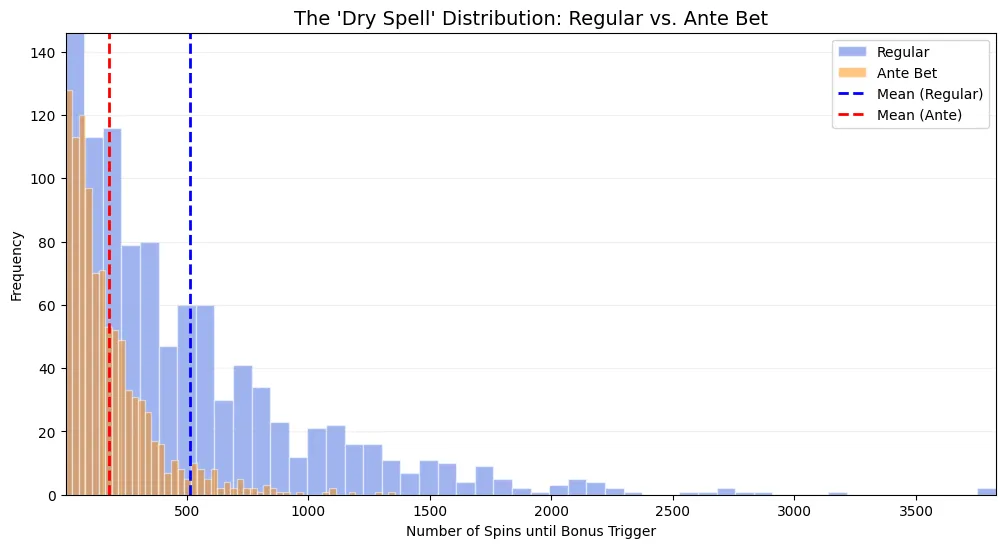
The chart is generated from the estimated probabilities. It is not a second independent sample from the game.
Why a bonus is never “due” under this model
For independent spins:
P(next spin triggers a bonus | previous losses) = pA sequence of 500 losing spins does not increase the probability that spin 501 triggers the feature. Believing that a win becomes more likely because of previous losses is the gambler’s fallacy.
Gates of Olympus RTP Results
Return to Player is estimated as:
RTP = total return / total wagerFor each normalized paid round, total_return contains the base-game result plus the final cumulative bonus result when that round triggered free spins.
def calculate_rtp(group: pd.DataFrame) -> float:
    total_wager = group["wager"].sum()
    total_return = group["total_return"].sum()

    if total_wager <= 0:
        raise ValueError("Total wager must be positive.")

    return 100 * total_return / total_wager


observed_rtp = (
    rounds.groupby("mode", observed=True)
    .apply(calculate_rtp, include_groups=False)
    .rename("observed_rtp_percent")
)

print(observed_rtp)
The observed values were:
Regular RTP: 89.263%
Ante RTP:   101.797%
The Ante result does not show that Ante mode has a positive expected value. It only shows that this sample returned more than it wagered during the observed period.
Why short-run RTP is unstable
Slot returns are strongly right-skewed. A typical sample contains:
- many zero-return spins;
- many small returns;
- fewer medium wins;
- a small number of large bonuses.
One unusually large payout can move the observed RTP by several percentage points.
The standard error of a sample mean decreases approximately as:
SE = standard deviation / sqrt(n)This means:
- halving uncertainty requires roughly four times as many observations;
- reducing uncertainty by a factor of ten requires roughly one hundred times as many observations.
Twenty thousand paid spins per mode can therefore remain imprecise for a high-volatility return distribution.
Bootstrap confidence intervals for RTP
def bootstrap_rtp(
    group: pd.DataFrame,
    n_bootstrap: int = 20_000,
    seed: int = 42,
) -> np.ndarray:
    if n_bootstrap <= 0:
        raise ValueError("n_bootstrap must be positive.")

    values = group[
        ["wager", "total_return"]
    ].to_numpy(dtype=float)

    if len(values) == 0:
        raise ValueError("Cannot bootstrap an empty group.")

    rng = np.random.default_rng(seed)
    estimates = np.empty(n_bootstrap)

    for index in range(n_bootstrap):
        sampled_indices = rng.integers(
            low=0,
            high=len(values),
            size=len(values),
        )

        sample = values[sampled_indices]
        estimates[index] = (
            100
            * sample[:, 1].sum()
            / sample[:, 0].sum()
        )

    return estimates


rtp_results = {}

for mode, group in rounds.groupby(
    "mode",
    observed=True,
):
    samples = bootstrap_rtp(group)

    rtp_results[mode] = {
        "estimate": calculate_rtp(group),
        "ci_low": np.percentile(samples, 2.5),
        "ci_high": np.percentile(samples, 97.5),
    }


print(pd.DataFrame(rtp_results).T)
The reproducible row-bootstrap results are:
| Mode | Observed RTP | 95% bootstrap interval |
|---|---|---|
| Regular | 89.263% | 78.52%–101.23% |
| Ante | 101.797% | 87.61%–117.85% |
The public game page lists 96.50%. That value lies inside both intervals.
The appropriate conclusion is:
This sample is too imprecise to distinguish either mode’s long-run RTP from 96.50% under the row-bootstrap model.
Failure to reject 96.50% does not prove that it is the exact theoretical RTP of the tested build.
Session-level bootstrap sensitivity check
The data was collected in 40 separate sessions. If observations within a session are more similar than observations across sessions, resampling individual rows can understate uncertainty.
A cluster bootstrap resamples whole sessions:
def cluster_bootstrap_rtp(
    group: pd.DataFrame,
    n_bootstrap: int = 10_000,
    seed: int = 42,
) -> np.ndarray:
    session_ids = group["session_id"].unique()

    if len(session_ids) < 2:
        raise ValueError(
            "At least two sessions are required."
        )

    sessions = {
        session_id: group[
            group["session_id"].eq(session_id)
        ]
        for session_id in session_ids
    }

    rng = np.random.default_rng(seed)
    estimates = np.empty(n_bootstrap)

    for index in range(n_bootstrap):
        sampled_sessions = rng.choice(
            session_ids,
            size=len(session_ids),
            replace=True,
        )

        wager_sum = sum(
            sessions[value]["wager"].sum()
            for value in sampled_sessions
        )
        return_sum = sum(
            sessions[value]["total_return"].sum()
            for value in sampled_sessions
        )

        estimates[index] = 100 * return_sum / wager_sum

    return estimates
The session-bootstrap intervals were approximately:
| Mode | 95% session-bootstrap interval |
|---|---|
| Regular | 78.89%–99.88% |
| Ante | 87.66%–116.33% |
The row and session bootstraps lead to the same broad conclusion: uncertainty remains large, and 96.50% is compatible with both samples.
Limits of the bootstrap
A bootstrap resamples outcomes that appeared in the data. It cannot invent an extremely rare payout that never occurred.
It also cannot correct:
- an incorrect wager denominator;
- duplicated or omitted bonus returns;
- missed spins;
- configuration changes;
- selective logging;
- dependence not captured by the resampling design.
Does Ante Bet Change Multiplier Behavior?
Multiplier analysis requires separating three questions:
- How often does a winning base spin include a positive multiplier?
- How large is the multiplier when such an event occurs?
- How much do multipliers contribute to return per paid spin?
This dataset directly supports the first two comparisons.
Multiplier-event frequency
Define a multiplier event as a paid base spin where:
base-game win > 0
and
recorded base multiplier > 0rounds["multiplier_event"] = (
rounds["win"].gt(0)
& rounds["base_multiplier"].gt(0)
)
multiplier_frequency = (
rounds.groupby("mode", observed=True)
["multiplier_event"]
.agg(["sum", "count", "mean"])
)
multiplier_frequency["percent"] = (
multiplier_frequency["mean"] * 100
)
print(multiplier_frequency)The observed rates were:
Regular: 295 / 20,000 = 1.475%
Ante:    346 / 20,000 = 1.730%
A two-sided Fisher exact test gives an unadjusted p-value of approximately:
p = 0.0464That is weak evidence of a frequency difference at a nominal 5% threshold. It is not robust to a reasonable correction for the multiple comparisons made in this article.
Conditional multiplier size
Among the paid base spins that produced a winning multiplier event:
| Metric | Regular | Ante |
|---|---|---|
| Event count | 295 | 346 |
| Mean multiplier | 13.26× | 12.60× |
| Median multiplier | 8× | 6× |
| Maximum recorded multiplier | 500× | 504× |
The maximum 504× value can occur when multiple multiplier symbols are combined.
The conventional two-sample Kolmogorov–Smirnov test gives:
KS statistic = 0.1004
Default/exact p-value = 0.0737
Explicit asymptotic p-value = 0.0755
Because multiplier values are discrete and contain many ties, a permutation calibration is also useful.
from scipy.stats import ks_2samp

regular_multipliers = (
    rounds.loc[
        rounds["mode"].eq("Regular")
        & rounds["multiplier_event"],
        "base_multiplier",
    ]
    .dropna()
    .to_numpy()
)

ante_multipliers = (
    rounds.loc[
        rounds["mode"].eq("Ante")
        & rounds["multiplier_event"],
        "base_multiplier",
    ]
    .dropna()
    .to_numpy()
)

observed_ks = ks_2samp(
    regular_multipliers,
    ante_multipliers,
).statistic

combined = np.concatenate([
    regular_multipliers,
    ante_multipliers,
])

regular_size = len(regular_multipliers)
rng = np.random.default_rng(seed=42)

n_permutations = 20_000
permuted_statistics = np.empty(n_permutations)

for index in range(n_permutations):
    shuffled = rng.permutation(combined)

    permuted_regular = shuffled[:regular_size]
    permuted_ante = shuffled[regular_size:]

    permuted_statistics[index] = ks_2samp(
        permuted_regular,
        permuted_ante,
    ).statistic

permutation_p_value = (
    1
    + np.count_nonzero(
        permuted_statistics >= observed_ks
    )
) / (n_permutations + 1)

print(f"Observed KS statistic: {observed_ks:.4f}")
print(f"Permutation p-value: {permutation_p_value:.6g}")
With the stated seed and 20,000 permutations, the permutation p-value is approximately:
p = 0.0328The asymptotic and permutation methods cross the 5% threshold in opposite directions. After accounting for the several tests performed in this study, neither multiplier comparison remains conventionally significant.
A careful conclusion is therefore:
The sample contains weak, method-sensitive evidence of multiplier differences, but it does not establish a robust Ante effect on multiplier behavior.
Non-significance is not proof of equality
A p-value above 0.05 means the study did not detect a difference under that test and threshold. It does not prove that two distributions are identical.
Demonstrating practical similarity requires an equivalence test with a predefined margin, such as:
- a maximum acceptable difference in multiplier-event probability;
- a maximum relative difference in mean multiplier contribution;
- a maximum acceptable shift in median multiplier.
Those margins should be chosen before examining the results.
Statistical Assumptions
The analysis relies on several assumptions.
Independent paid rounds
Each paid round is treated as independent of previous rounds. This assumption underlies the geometric dry-spell model and the inferential comparisons.
Stable game configuration
The probability model is assumed not to change during collection. That requires a stable:
- game version;
- RTP configuration;
- wager mode;
- feature configuration;
- collection process.
Representative logging
The collector must not selectively miss:
- zero-return spins;
- large wins;
- bonus triggers;
- retriggers;
- interrupted sequences;
- particular animation states.
Strong right skew
The return distribution contains many small or zero outcomes and a small number of large outcomes. Because the game has a finite maximum payout, the distribution is not literally unbounded, but it is strongly right-skewed and dominated by rare events.
Limitations of the 40,000-Spin Analysis
Demo data
The collection came from demo play. The study did not independently verify that every real-money deployment uses the same configuration or random process.
Exact RTP configuration
The public game page lists 96.50%, but the exact help-screen RTP for the tested build should be archived with the project.
Bonus reconstruction
This file stores cumulative bonus totals, so only the final value in each sequence is used. A collector with incremental bonus rows would require a different rule.
Rare outcomes
A sample can entirely miss low-probability, high-impact payouts. This makes precise RTP verification difficult even with tens of thousands of spins.
Browser automation
Animation timing, disconnections, duplicate events, and missed state transitions can introduce measurement error.
Session effects
Systematic differences between sessions can violate the assumption that all paid rounds come from one stable distribution.
Multiple testing
This study examines bonus frequency, the exact rate ratio, RTP, multiplier-event frequency, and multiplier size. Multiple comparisons increase the chance of a false-positive result.
No independent certification
The analysis does not inspect or certify the game’s source code, RNG implementation, mathematical model, or regulator reports.
What 40,000 Spins Can and Cannot Tell Us
A 40,000-paid-spin dataset is useful for:
- detecting a large difference in common event rates;
- estimating approximate bonus waiting times;
- illustrating short-run RTP volatility;
- finding obvious data-cleaning problems;
- comparing broad sample patterns.
It is much weaker for:
- verifying an exact theoretical RTP;
- estimating rare maximum-win probabilities;
- detecting small distributional differences;
- generalizing to configurations that were not sampled;
- making claims about internal RNG implementation.
A larger sample improves precision, but sample size cannot repair incorrect logging or an invalid observational unit.
Final Conclusions
Ante increased the observed bonus frequency
Regular mode produced 39 bonus triggers in 20,000 paid spins, compared with 112 triggers in Ante mode.
The observed rates were 0.195% and 0.560%, and equal rates were strongly rejected.
The sample is narrowly compatible with the advertised 2× claim
The observed lift was 2.872×, with a 95% confidence interval of approximately 1.996× to 4.132×.
The direct p-value against an exact 2× ratio was 0.0513. The result does not justify claiming that the true lift is greater than 2×.
Short-run RTP was highly unstable
The observed RTP values were 89.263% for Regular and 101.797% for Ante.
Both bootstrap intervals were wide and included 96.50%, so the sample cannot precisely verify or reject that theoretical value.
Multiplier evidence was weak and method-dependent
Ante produced slightly more winning base spins with a multiplier, while Regular had a higher median multiplier among those events.
Individual unadjusted tests produced borderline results, but the overall evidence was not robust after considering multiple testing and the discreteness of the multiplier data.
Frequently Asked Questions
What is the published RTP of Gates of Olympus?
Pragmatic Play’s public game page lists 96.50% for the standard Gates of Olympus game. The exact RTP shown in the tested build should still be recorded because configurations can vary.
What RTP did the 40,000-spin sample produce?
The observed RTP was 89.263% for Regular mode and 101.797% for Ante mode. These are sample outcomes, not estimates precise enough to define the game’s true long-run RTP.
Does 96.5% RTP mean I receive €96.50 for every €100 wagered?
No. RTP is a long-run average across a very large number of wagers. A player or short session can finish far above or below that percentage.
How often did the Gates of Olympus bonus trigger?
The sample recorded 39 Regular bonuses in 20,000 paid spins and 112 Ante bonuses in 20,000 paid spins. The observed rates were 0.195% and 0.560%.
Did Ante Bet double the bonus chance?
The observed lift was about 2.87×. However, the confidence interval was wide, and a direct test against an exact 2× rate ratio produced p = 0.0513. The sample is therefore narrowly compatible with a true doubling.
How many spins did it take to trigger a bonus?
Based on the observed rates, the estimated mean wait was about 513 Regular spins and 179 Ante spins. These are averages, not guarantees.
Can a bonus take more than 1,000 spins?
Yes. Under the geometric model fitted to this sample, the probability of a Regular wait exceeding 1,000 spins was about 14.2%. The corresponding Ante estimate was about 0.364%.
Is a bonus more likely after a long losing streak?
Not under an independent-spin model. Previous losses do not make the next bonus due.
Is 40,000 spins enough to verify RTP?
It is enough to produce a useful estimate, but not enough to verify a high-volatility game’s exact theoretical RTP precisely. Rare large payouts dominate the uncertainty.
Why use a bootstrap confidence interval?
The bootstrap estimates sampling uncertainty without assuming a normally distributed payout. It still depends on the observed rounds being representative and cannot reproduce rare outcomes that never appeared.
Does Ante Bet guarantee more profit?
No. A higher bonus-trigger frequency does not imply a positive expected value, remove volatility, or guarantee a profit.
Can this analysis prove the game is fair?
No. Output analysis cannot replace certified game mathematics, source-code inspection, RNG testing, or regulatory reports.
Key Takeaways
- Use one row per paid wager when estimating RTP.
- Attach each cumulative bonus total to the paid round that triggered it.
- Include the full
0.25Ante wager in the RTP denominator. - Publish exact event counts, not only rounded percentages.
- Test the advertised
2×claim with a rate ratio, not only an equal-rates test. - Use the geometric distribution to quantify bonus dry-spell risk.
- Interpret an RTP confidence interval against a specified theoretical value.
- Treat bootstrap intervals cautiously when rare outcomes are absent.
- Separate multiplier frequency from conditional multiplier size.
- Correct for multiple testing when several related hypotheses are examined.
- Do not interpret a non-significant result as proof of equality.
- Describe the work as observational analysis rather than a certified audit.
The dataset cannot predict the next spin. It shows how long losing sequences, occasional large payouts, unstable short-run RTP, and uncertain mode comparisons can all arise from the same high-variance probability model.