Sweet Bonanza 1000 RTP Analysis: 60,000 Spins
Python analysis of 60,000 Sweet Bonanza 1000 demo spins, covering RTP, dead spins, bonus frequency, payout concentration, and logging errors.

What happened across 60,000 paid demo spins of Sweet Bonanza 1000?
After reconstructing every bonus and reducing the log to one row per paid wager, the sample produced an observed RTP of 109.05%, a zero-return paid-round rate of 56.64%, and 131 bonus triggers. The published 96.53% RTP remained inside both the paid-round and session-cluster bootstrap intervals.
Those results do not prove that the game has a positive expected value or certify its fairness. The sample return was dominated by rare outcomes, including one bonus worth more than 5,000× the triggering wager.
This chapter uses Python to answer five questions:
- How often did a paid round return zero?
- How concentrated was the observed return?
- How frequently did the bonus trigger, and what did it pay?
- What do the recorded multiplier fields actually measure?
- Was the sample RTP statistically compatible with the published RTP?
Responsible-gambling note: RTP is a long-run mathematical expectation, not a promise for one session. A sample can return more than 100% even when the underlying expected value is below 100%.
Key Results from the Supplied Dataset
| Metric | Recalculated result |
|---|---|
| Raw logged events | 61,455 |
| Paid spins | 60,000 |
| Recorded free-spin rows | 1,455 |
| Collection sessions | 60 |
| Bonus sessions | 131 |
| Zero-return paid rounds | 33,981 |
| Dead-spin rate | 56.635% |
| 95% Wilson interval for dead-spin rate | 56.238%–57.031% |
| Bonus-trigger rate | 0.2183% |
| Approximate mean paid spins per trigger | 458 |
| Median bonus return | 10.41 currency units / 52.05× bet |
| Largest 10% of winning paid rounds: share of return | 57.401% |
| 95% bootstrap interval for top-10% share | 50.826%–64.767% |
| Total wager | 12,000.00 |
| Normalized total return | 13,086.14 |
| Observed RTP | 109.051% |
| 95% paid-round bootstrap interval for RTP | 94.318%–132.566% |
| 95% session-cluster bootstrap interval for RTP | 93.881%–131.662% |
The supplied file contains only Regular-mode observations:
is_ante = False for all 61,455 rows
bet = 0.20 for all rows
No Regular-versus-Ante comparison can be made from this dataset.
Corrections to the Earlier Results
Recalculating the article from the supplied CSV changed several results.
| Earlier figure | Recalculated figure | Reason |
|---|---|---|
| 56.74% dead spins | 56.635% | The earlier value counted zero-base-return bonus triggers as dead, even though their paid rounds later returned a bonus payout. |
| 73.486% from the largest 10% of wins | 57.401% | The earlier calculation treated repeated cumulative bonus totals as separate winning observations. |
| 59.77% ineffective multipliers | Not a valid game-mechanic estimate | All 87 supposed base-game multiplier rows occurred immediately after a bonus and appear to be collector-state leakage. |
| 108.81% observed RTP | 109.051% | Reconstructing all 131 cumulative bonus sessions and attaching each final value to its triggering paid spin produces 109.051%. |
| 93.99%–130.76% RTP interval | 94.318%–132.566% | Recalculated with 20,000 paid-round bootstrap samples and seed 42. |
The earlier 108.81% RTP could not be reproduced exactly from the supplied file. The normalized calculation is fully accounted for:
Base-game return:       9,292.22
Final bonus returns:    3,793.92
Total return:          13,086.14
Total wager:           12,000.00
Observed RTP:            109.051%
Table of Contents
- Official Sweet Bonanza 1000 Information
- What the Dataset Contains
- How the Raw Events Were Normalized
- Dead-Spin Analysis
- Return-Concentration Analysis
- Bonus-Frequency and Payout Analysis
- Multiplier Logging Analysis
- RTP and Bootstrap Analysis
- Limitations
- Frequently Asked Questions
Official Sweet Bonanza 1000 Information
Pragmatic Play’s public Sweet Bonanza 1000 page lists:
- a 6×5 layout;
- wins when eight or more matching fruit or candy symbols land;
- tumbling wins;
- a maximum advertised win of
25,000×; - 10 free spins from at least four lollipop symbols;
- candy-bomb multipliers up to
1,000×in the bonus game; - five additional free spins from at least three lollipops during the feature;
- a published RTP of
96.53%.
Official source: Pragmatic Play — Sweet Bonanza 1000, checked July 11, 2026.
The exact RTP and rules shown in the tested demo build should still be archived. Public product pages do not prove that every market or operator uses one identical configuration.
How Sweet Bonanza 1000 Works
Anywhere-Pays Wins
A payout occurs when at least eight matching symbols appear anywhere on the 6×5 grid. They do not need to occupy adjacent positions or a conventional payline.
Tumbles
After a win:
- the winning symbols disappear;
- new symbols fall into the empty positions;
- another win may form;
- the sequence continues until no further win occurs.
One paid spin can therefore contain several dependent tumbles. The paid round—not an individual tumble—is the correct unit for RTP.
Bonus Multipliers
The public rules place candy-bomb multipliers in the bonus game. During a tumble, multiplier values remain visible and are added before being applied to the qualifying win.
A reliable multiplier study requires tumble-level fields showing:
- which tumble displayed the multiplier;
- whether that same tumble produced a qualifying win;
- the multiplier value applied;
- the tumble payout.
The supplied dataset contains only one aggregate multiplier_total field per logged row. It cannot independently reconstruct the full multiplier mechanism.
This Is a Statistical Analysis, Not a Fairness Certification
The dataset contains outputs collected from demo play. It does not provide:
- source code;
- certified probability tables;
- RNG output or seeds;
- regulator-controlled testing;
- every available RTP configuration;
- proof that demo and real-money deployments are identical.
The analysis can describe the supplied sample, expose logging problems, quantify uncertainty, and test reproducible statistical claims. It cannot certify the game or predict future spins.
What the Dataset Contains
The supplied CSV has seven columns:
| Column | Meaning in this analysis |
|---|---|
round_id | Event counter that restarts at the beginning of each collection session |
bet | Recorded wager; always 0.20 in this file |
win | Base return on paid rows and cumulative feature return on bonus rows |
cascade_depth | Recorded number of tumbles or cascades |
multiplier_total | Aggregate multiplier field recorded by the collector |
is_bonus | Whether the row belongs to a free-spin sequence |
is_ante | Ante flag; always False in this file |
The round_id resets reveal 60 collection sessions. Every session contains exactly 1,000 paid rows plus any free-spin rows generated during that session.
from __future__ import annotations

import numpy as np
import pandas as pd

raw = pd.read_csv("dataset.csv")

raw["session_id"] = (
    raw["round_id"]
    .diff()
    .fillna(1)
    .le(0)
    .cumsum()
)

print(raw.shape)
print(raw["session_id"].nunique())
print((~raw["is_bonus"]).sum())
print(raw["is_bonus"].sum())
Expected output:
Rows:              61,455
Sessions:               60
Paid rows:          60,000
Bonus rows:          1,455
How the Raw Events Were Normalized
One Row per Paid Wager
For RTP, dead-spin rate, payout concentration, and bonus frequency, the observational unit is one paid wager:
paid-round return
    = base-game return
    + final cumulative bonus return caused by that wager
The bonus rows cannot be summed because their win values are cumulative.
For example, one recorded feature progressed as follows:
0.60, 0.60, 0.60, 9.18, 9.28, 9.28, 9.28, 9.28, 9.28, 9.28Its feature return is 9.28, not the sum of all ten rows.
Every one of the 131 bonus sequences in the file has a non-decreasing win series, supporting the cumulative interpretation.
Reconstruct the Bonus Sessions
raw = raw.reset_index(names="event_index")

previous_bonus_state = (
    raw.groupby("session_id", observed=True)["is_bonus"]
    .shift(fill_value=False)
)

raw["bonus_start"] = (
    raw["is_bonus"]
    & ~previous_bonus_state
)

raw["bonus_id"] = (
    raw["bonus_start"]
    .cumsum()
    .where(raw["is_bonus"])
)

bonus_rows = raw[raw["is_bonus"]].copy()

bonus_monotonic = (
    bonus_rows.groupby("bonus_id", observed=True)["win"]
    .apply(lambda values: values.is_monotonic_increasing)
)

if not bonus_monotonic.all():
    raise ValueError(
        "At least one bonus sequence is not cumulative."
    )

bonuses = (
    bonus_rows.groupby("bonus_id", observed=True)
    .agg(
        session_id=("session_id", "first"),
        first_event=("event_index", "min"),
        last_event=("event_index", "max"),
        free_spin_rows=("event_index", "size"),
        bonus_return=("win", "last"),
    )
    .reset_index()
)

bonuses["trigger_event"] = (
    bonuses["first_event"] - 1
)
Attach Each Bonus to Its Triggering Paid Spin
paid_rounds = raw.loc[
    ~raw["is_bonus"],
    [
        "event_index",
        "session_id",
        "round_id",
        "bet",
        "win",
    ],
].copy()

paid_rounds = paid_rounds.rename(
    columns={
        "bet": "wager",
        "win": "base_return",
    }
)

bonus_map = bonuses.set_index(
    "trigger_event"
)["bonus_return"]

paid_rounds["bonus_return"] = (
    paid_rounds["event_index"]
    .map(bonus_map)
    .fillna(0.0)
)

paid_rounds["bonus_triggered"] = (
    paid_rounds["bonus_return"].gt(0)
)

paid_rounds["total_return"] = (
    paid_rounds["base_return"]
    + paid_rounds["bonus_return"]
)

paid_rounds["paid_round_id"] = np.arange(
    len(paid_rounds)
)
Validate the Reconstruction
assert len(raw) == 61_455
assert len(paid_rounds) == 60_000
assert len(bonuses) == 131
assert raw["session_id"].nunique() == 60
assert paid_rounds["wager"].eq(0.20).all()
assert not raw["is_ante"].any()
assert paid_rounds["paid_round_id"].is_unique
assert paid_rounds["total_return"].ge(0).all()

assert np.isclose(
    paid_rounds["base_return"].sum(),
    9_292.22,
)

assert np.isclose(
    bonuses["bonus_return"].sum(),
    3_793.92,
)

assert np.isclose(
    paid_rounds["total_return"].sum(),
    13_086.14,
)
Statistical Assumptions
The following analyses assume:
Independent Paid Rounds
Paid rounds are treated as independent observations. Tumbles and free spins inside one paid round are not treated as independent wagers.
Stable Configuration
The game build, denomination, RTP setting, collection logic, and feature rules are assumed not to have changed during collection.
Complete Logging
The collector is assumed to have captured zero-return rounds, bonus starts, retriggers, large wins, and session resets without selective omissions.
Representative Empirical Distribution
The bootstrap treats the observed rounds or sessions as representative. It cannot generate rare outcomes absent from the sample.
Question 1: How Common Were Dead Spins?
A dead spin is defined here as a normalized paid round whose complete attributable return equals zero:
total_return = 0This definition prevents a zero-base-return spin that triggers a paying bonus from being classified as dead.
paid_rounds["dead_spin"] = (
    paid_rounds["total_return"].eq(0)
)

number_dead = int(
    paid_rounds["dead_spin"].sum()
)

number_paid = len(paid_rounds)

dead_rate = number_dead / number_paid
The supplied data produced:
Dead paid rounds: 33,981 / 60,000
Dead-spin rate:    56.635%
Wilson Confidence Interval
from statsmodels.stats.proportion import (
    proportion_confint,
)

ci_low, ci_high = proportion_confint(
    count=number_dead,
    nobs=number_paid,
    alpha=0.05,
    method="wilson",
)

print(f"Rate: {dead_rate:.4%}")
print(f"95% Wilson CI: {ci_low:.4%}–{ci_high:.4%}")
Output:
Rate: 56.6350%
95% Wilson CI: 56.2380%–57.0311%
Why the Earlier Result Was 56.74%
The raw paid rows contain 34,046 observations with base_return = 0, or 56.7433%.
However, 65 of those rows triggered a bonus and therefore had a positive normalized total_return. Counting them as dead mixes the base-spin outcome with the complete paid-round outcome.
Both statistics can be reported, but they answer different questions:
| Definition | Estimate |
|---|---|
| Base-game return equals zero | 56.743% |
| Complete paid-round return equals zero | 56.635% |
Test Against a 50% Benchmark
A one-sided exact binomial test gives:
from scipy.stats import binomtest

dead_test = binomtest(
    k=number_dead,
    n=number_paid,
    p=0.50,
    alternative="greater",
)

print(dead_test.pvalue)
p = 1.10 × 10^-232The result is unsurprising with 60,000 observations. Estimation and practical interpretation are more useful than testing an arbitrary 50% threshold.
Session-Level Variation
session_dead_rates = (
    paid_rounds.groupby(
        "session_id",
        observed=True,
    )["dead_spin"]
    .mean()
)

print(session_dead_rates.describe())
Across the 60 sessions, the dead-spin rate ranged from:
Minimum: 51.9%
Median:  56.7%
Maximum: 60.2%
The pooled interval is narrow because it contains 60,000 paid rounds. It does not imply that every 1,000-spin session will have nearly the same rate.
Question 2: How Concentrated Was the Return?
Return concentration measures how much of the observed payout came from the largest winning paid rounds.
The correct input is the normalized total_return, not every raw bonus snapshot.
winning_rounds = (
    paid_rounds.loc[
        paid_rounds["total_return"].gt(0),
        "total_return",
    ]
    .sort_values(ascending=False)
    .reset_index(drop=True)
)

number_top = max(
    1,
    int(np.ceil(0.10 * len(winning_rounds))),
)

top_share = (
    winning_rounds.iloc[:number_top].sum()
    / winning_rounds.sum()
)

print(len(winning_rounds))
print(number_top)
print(top_share)
Output:
Winning paid rounds:             26,019
Largest 10% of winning rounds:    2,602
Share of normalized return:      57.401%
Why the Earlier Figure Was 73.486%
The 73.486% result is reproducible only when all positive raw win rows are treated as independent observations.
That method includes multiple cumulative values from the same bonus:
0.60, 0.60, 0.60, 9.18, 9.28, 9.28, ...Those are not separate paid-round returns. They repeatedly count one evolving feature total and inflate the apparent concentration.
Bootstrap Interval for the Top-10% Share
def bootstrap_top_share(
    returns: np.ndarray,
    fraction: float = 0.10,
    n_bootstrap: int = 20_000,
    seed: int = 42,
    batch_size: int = 1_000,
) -> np.ndarray:
    if not 0 < fraction <= 1:
        raise ValueError(
            "fraction must be between 0 and 1."
        )

    values, counts = np.unique(
        returns,
        return_counts=True,
    )

    order = np.argsort(values)[::-1]
    values = values[order]
    probabilities = counts[order] / counts.sum()

    positive_mask = values > 0
    positive_values = values[positive_mask]

    if len(positive_values) == 0:
        raise ValueError(
            "At least one positive return is required."
        )

    rng = np.random.default_rng(seed)
    estimates = np.empty(n_bootstrap)
    number_rounds = len(returns)

    for start in range(0, n_bootstrap, batch_size):
        stop = min(
            start + batch_size,
            n_bootstrap,
        )

        sampled_counts = rng.multinomial(
            number_rounds,
            probabilities,
            size=stop - start,
        )

        positive_counts = sampled_counts[
            :, positive_mask
        ]

        number_positive = positive_counts.sum(axis=1)
        number_top = np.ceil(
            fraction * number_positive
        ).astype(int)

        cumulative_counts = np.cumsum(
            positive_counts,
            axis=1,
        )

        cumulative_returns = np.cumsum(
            positive_counts * positive_values,
            axis=1,
        )

        cutoff = (
            cumulative_counts >= number_top[:, None]
        ).argmax(axis=1)

        row_index = np.arange(stop - start)

        previous_count = np.where(
            cutoff > 0,
            cumulative_counts[
                row_index,
                np.maximum(cutoff - 1, 0),
            ],
            0,
        )

        previous_return = np.where(
            cutoff > 0,
            cumulative_returns[
                row_index,
                np.maximum(cutoff - 1, 0),
            ],
            0.0,
        )

        top_return = (
            previous_return
            + (number_top - previous_count)
            * positive_values[cutoff]
        )

        total_return = (
            positive_counts * positive_values
        ).sum(axis=1)

        estimates[start:stop] = (
            top_return / total_return
        )

    return estimates

share_samples = bootstrap_top_share(
    paid_rounds["total_return"].to_numpy()
)

share_ci = np.percentile(
    share_samples,
    [2.5, 97.5],
)
Using 20,000 resamples and seed 42:
Observed share:   57.401%
95% bootstrap CI: 50.826%–64.767%
Plot the Concentration Curve
import matplotlib.pyplot as plt

ordered = winning_rounds.to_numpy()

cumulative_share = (
    np.cumsum(ordered)
    / ordered.sum()
)

fraction_of_winners = (
    np.arange(1, len(ordered) + 1)
    / len(ordered)
)

plt.figure(figsize=(10, 6))
plt.plot(
    fraction_of_winners,
    cumulative_share,
)
plt.axvline(
    0.10,
    linestyle="--",
    label="Largest 10% of winning paid rounds",
)
plt.axhline(
    top_share,
    linestyle="--",
    label=f"Return share: {top_share:.1%}",
)
plt.xlabel("Fraction of winning paid rounds")
plt.ylabel("Fraction of normalized return")
plt.title(
    "Sweet Bonanza 1000 Paid-Round Return Concentration"
)
plt.legend()
plt.tight_layout()
plt.show()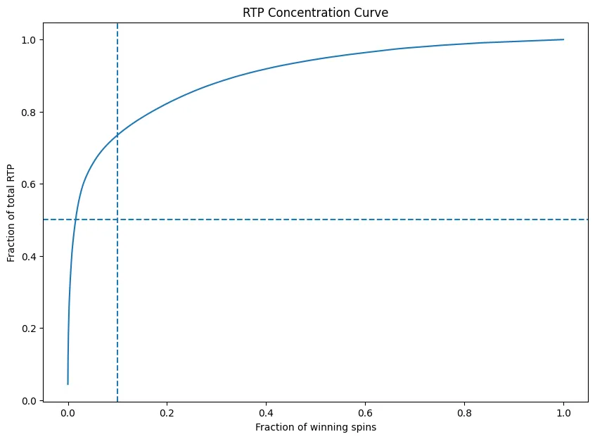
The result shows substantial concentration, but less than the raw-row calculation suggested. A small subset of wins still had a large influence on the sample mean.
Question 3: How Often Did the Bonus Trigger?
The normalized dataset contains 131 bonus sessions from 60,000 paid spins.
bonus_count = int(
    paid_rounds["bonus_triggered"].sum()
)

paid_count = len(paid_rounds)

bonus_rate = bonus_count / paid_count

bonus_ci = proportion_confint(
    count=bonus_count,
    nobs=paid_count,
    alpha=0.05,
    method="wilson",
)
Results:
Bonus triggers:              131
Trigger rate:                0.2183%
95% Wilson interval:         0.1840%–0.2590%
Mean paid spins per trigger: 458.0
Gross wager per trigger:     91.60
The mean waiting estimate is:
1 / 0.0021833 = 458.0 paid spinsThis is an average, not a deadline. It does not mean the feature becomes due after 458 spins.
Bonus Length and Retriggers
The 131 recorded bonus sequences contained:
| Recorded free-spin rows | Number of bonus sessions |
|---|---|
| 10 | 107 |
| 15 | 20 |
| 20 | 3 |
| 25 | 1 |
This pattern is consistent with initial 10-spin features and five-spin retriggers, assuming one bonus row represents one free spin.
Bonus-Payout Distribution
bonuses["bonus_return_multiple"] = (
    bonuses["bonus_return"] / 0.20
)

bonus_summary = bonuses[
    ["bonus_return", "bonus_return_multiple"]
].describe(
    percentiles=[0.10, 0.25, 0.50, 0.75, 0.90]
)

print(bonus_summary)| Statistic | Currency units | Bet multiple |
|---|---|---|
| Minimum | 0.70 | 3.50× |
| 10th percentile | 2.47 | 12.35× |
| 25th percentile | 5.635 | 28.175× |
| Median | 10.41 | 52.05× |
| Mean | 28.961 | 144.806× |
| 75th percentile | 23.465 | 117.325× |
| 90th percentile | 44.78 | 223.90× |
| Maximum | 1,096.36 | 5,481.80× |
The mean is almost three times the median because a small number of large features pull it upward.
Additional descriptive results:
Bonuses below 50× bet:  46.56%
Bonuses below 100× bet: 69.47%
Bonus-only share of all normalized return: 28.99%
Why 91.60 Is Not a Bonus Price
The observed gross wager per trigger is:
12,000 total wager / 131 triggers = 91.60It is not:
- a fixed feature-purchase price;
- the net amount lost before the bonus;
- the expected cost of one feature;
- directly comparable with a median feature payout as a profitability test.
The paid spins before each trigger also produced base-game returns.
The earlier sign-test framing can be reproduced: 127 of 131 bonus payouts were below 91.60, producing a one-sided exact binomial p-value of approximately 4.44 × 10^-33. That test does not establish that the bonus is unprofitable because the comparison threshold is an estimated gross-wager average and excludes base returns earned during the wait.
Better Bonus-Economics Measures
More useful descriptive statistics include:
- trigger probability;
- median and mean bonus return in wager multiples;
- feature-return quantiles;
- bonus contribution to total return;
- complete trigger-to-trigger episode returns.
A trigger-to-trigger episode should include every wager and every return between two observed triggers in the same uninterrupted collection session.
Question 4: What Do the Multiplier Records Mean?
The earlier analysis identified 87 non-bonus rows where:
multiplier_total > 0Of those rows, 52 had win = 0, producing:
52 / 87 = 59.770%A normal-approximation one-sided test gives the earlier p-value of approximately 0.0342. An exact binomial test gives:
One-sided exact p-value: 0.04284
95% exact interval:      48.71%–70.15%
95% Wilson interval:     49.26%–69.45%
However, the structural inspection is more important than the p-value.
All 87 Rows Followed a Bonus Immediately
suspected_rows = raw.loc[
    ~raw["is_bonus"]
    & raw["multiplier_total"].gt(0)
].copy()

previous_row_was_bonus = (
    raw["is_bonus"]
    .shift(fill_value=False)
    .loc[suspected_rows.index]
    .to_numpy()
)

print(len(suspected_rows))
print(previous_row_was_bonus.sum())
Output:
Non-bonus rows with multiplier_total > 0: 87
Those immediately following a bonus row: 87
Every supposed base-game multiplier event occurred on the first paid row after a bonus sequence.
The official public rules place candy-bomb multipliers in the bonus game. The pattern strongly suggests that multiplier_total was not cleared immediately when the collector left bonus mode.
Therefore, 59.77% should be treated as a logging-state diagnostic, not an estimate of how often real multiplier symbols have no economic effect.
What Would Be Needed for a Valid Multiplier Test?
A valid study requires one row per tumble with fields such as:
paid_round_id
bonus_id
free_spin_index
tumble_index
symbol_win
multiplier_landed
multiplier_value
multiplier_applied
tumble_return
Without those fields, the dataset cannot establish whether a multiplier landed on the same tumble as a qualifying win.
Question 5: Was the Observed RTP Compatible with 96.53%?
RTP is calculated from normalized paid rounds:
RTP = total return / total wagerdef calculate_rtp(
group: pd.DataFrame,
) -> float:
total_wager = group["wager"].sum()
total_return = group["total_return"].sum()
if total_wager <= 0:
raise ValueError(
"Total wager must be positive."
)
return 100 * total_return / total_wager
observed_rtp = calculate_rtp(paid_rounds)The supplied dataset produced:
Total wager:  12,000.00
Total return: 13,086.14
Observed RTP: 109.051%
The sample finished in profit. That does not imply a positive long-run expectation.
Paid-Round Bootstrap
The nonparametric bootstrap resamples normalized paid rounds with replacement.
def bootstrap_rtp_constant_wager(
    group: pd.DataFrame,
    n_bootstrap: int = 20_000,
    seed: int = 42,
    batch_size: int = 1_000,
) -> np.ndarray:
    wagers = group["wager"].to_numpy(dtype=float)
    returns = group["total_return"].to_numpy(dtype=float)

    if len(group) == 0:
        raise ValueError(
            "Cannot bootstrap an empty dataset."
        )

    if not np.allclose(wagers, wagers[0]):
        raise ValueError(
            "This efficient implementation requires "
            "a constant wager."
        )

    values, counts = np.unique(
        returns,
        return_counts=True,
    )

    probabilities = counts / counts.sum()
    number_rounds = len(group)
    total_wager = number_rounds * wagers[0]

    rng = np.random.default_rng(seed)
    estimates = np.empty(n_bootstrap)

    for start in range(0, n_bootstrap, batch_size):
        stop = min(
            start + batch_size,
            n_bootstrap,
        )

        sampled_counts = rng.multinomial(
            number_rounds,
            probabilities,
            size=stop - start,
        )

        sampled_return = sampled_counts @ values

        estimates[start:stop] = (
            100 * sampled_return / total_wager
        )

    return estimates

rtp_samples = bootstrap_rtp_constant_wager(
    paid_rounds
)

row_ci = np.percentile(
    rtp_samples,
    [2.5, 97.5],
)
Using 20,000 resamples and seed 42:
Observed RTP: 109.051%
95% interval: 94.318%–132.566%
The published 96.53% value lies inside this interval.
Under this empirical bootstrap model, the sample does not provide strong evidence against 96.53%. The interval is also wide enough to include many other values, so this is not confirmation of the theoretical RTP.
Session-Cluster Bootstrap
Paid rounds from one browser session may share collection conditions. A sensitivity analysis can resample complete sessions instead of individual rounds.
def cluster_bootstrap_rtp(
    group: pd.DataFrame,
    n_bootstrap: int = 20_000,
    seed: int = 42,
) -> np.ndarray:
    sessions = (
        group.groupby(
            "session_id",
            observed=True,
        )
        .agg(
            wager=("wager", "sum"),
            total_return=("total_return", "sum"),
        )
        .reset_index(drop=True)
    )

    if len(sessions) < 2:
        raise ValueError(
            "At least two sessions are required."
        )

    rng = np.random.default_rng(seed)

    indices = rng.integers(
        low=0,
        high=len(sessions),
        size=(n_bootstrap, len(sessions)),
    )

    wagers = sessions["wager"].to_numpy()
    returns = sessions["total_return"].to_numpy()

    return (
        100
        * returns[indices].sum(axis=1)
        / wagers[indices].sum(axis=1)
    )

cluster_samples = cluster_bootstrap_rtp(
    paid_rounds
)

cluster_ci = np.percentile(
    cluster_samples,
    [2.5, 97.5],
)
Result:
95% session-cluster interval: 93.881%–131.662%The similarity between the row and session intervals suggests that session-level resampling does not materially change the broad conclusion.
Session RTP Was Highly Variable
Each session contained 1,000 paid spins. Their observed RTP values ranged from:
Minimum: 71.455%
Median:  91.343%
Maximum: 640.735%
The maximum came from a session containing an exceptionally large bonus. This illustrates how one rare outcome can dominate a limited sample.
Why the Bootstrap Is Still Limited
The empirical bootstrap cannot create a payout that never occurred in the dataset.
If the true game includes extremely rare high-impact outcomes absent from the sample, the bootstrap may understate long-run uncertainty. It also cannot correct:
- missing events;
- duplicated events;
- an incorrect wager denominator;
- changing game configurations;
- incorrect bonus reconstruction;
- non-representative collection sessions.
Mean Return vs. Typical Experience
The observed mean determines RTP:
mean paid-round return = 0.218102
wager per paid round   = 0.20
The median paid-round return was zero.
That is not a contradiction. A large number of zero and small returns can coexist with a high mean when a few outcomes are very large.
The sample’s largest normalized paid-round return was approximately:
1,096.97 currency unitsOne outcome of that size has a visible effect on the average of 60,000 spins.
What 60,000 Spins Can and Cannot Tell Us
The Dataset Can Estimate
- the observed paid-round dead-spin rate;
- the observed bonus-trigger rate;
- feature-payout quantiles;
- return concentration;
- sample RTP;
- session-to-session variation;
- collector anomalies visible in the logged fields.
The Dataset Cannot Prove
- the internal RNG is fair;
- the exact theoretical RTP;
- the probability of unobserved rare outcomes;
- demo and real-money equivalence;
- every operator uses the same configuration;
- the next spin’s result;
- the true multiplier mechanism without tumble-level records.
Main Limitations
Demo Environment
The data came from demo play. The article does not independently verify that every real-money deployment uses the same configuration.
No Ante Sample
All is_ante values are false. The dataset cannot estimate the effect of an Ante or double-chance mode.
Inferred Sessions
Session identifiers were reconstructed from round_id resets rather than supplied explicitly.
Cumulative Bonus Field
Bonus win values are cumulative. The normalization uses each feature’s final row, which is strongly supported by the non-decreasing sequences but should still be documented by the collector’s author.
Aggregate Multiplier Field
The dataset lacks tumble-level multiplier data. The 87 non-bonus multiplier rows appear to be transition-state leakage.
Rare Outcomes
A 25,000× advertised maximum is far above most observed outcomes. Sixty thousand spins can still miss important low-probability events.
Bootstrap Assumptions
The bootstrap assumes the observed rounds or sessions are representative and exchangeable. It cannot reconstruct missing tail outcomes.
No Independent Certification
The analysis does not inspect source code, certified game mathematics, RNG output, or regulator reports.
Final Conclusions
1. More Than Half of Paid Rounds Returned Zero
The normalized dead-spin rate was 56.635%, with a 95% Wilson interval of 56.238%–57.031%.
The earlier 56.74% figure measured zero base returns and included 65 rounds that later returned a bonus payout.
2. Return Was Concentrated, but Less Than Originally Reported
The largest 10% of winning paid rounds generated 57.401% of normalized return.
The earlier 73.486% result was inflated by repeated cumulative bonus snapshots.
3. The Sample Recorded 131 Bonus Triggers
The observed trigger rate was 0.2183%, or approximately one trigger per 458 paid spins.
The median feature returned 52.05× the wager, while the mean was 144.81× because rare large features pulled it upward.
4. The Multiplier Result Was a Logging Artifact
The earlier 59.77% estimate can be reproduced numerically, but every included row occurred immediately after a bonus sequence.
It should not be interpreted as evidence about the actual multiplier mechanic.
5. The Sample RTP Was 109.051%
The normalized sample returned 13,086.14 from 12,000.00 wagered.
Both the paid-round and session-cluster bootstrap intervals included the published 96.53% RTP. The sample therefore did not reject that value, but its uncertainty was too wide to verify it precisely.
Frequently Asked Questions
What was the observed Sweet Bonanza 1000 RTP in this dataset?
The normalized observed RTP was 109.051%, based on 13,086.14 returned from 12,000.00 wagered.
Why is this different from the earlier 108.81% result?
The earlier figure could not be reproduced exactly. Using all 60,000 paid wagers and the final cumulative return from each of the 131 bonus sessions produces 109.051%.
Does an RTP above 100% mean the game is profitable?
No. It means this limited sample returned more than it wagered. Negative-expectation games can produce profitable sessions or samples through random variation.
What is the published Sweet Bonanza 1000 RTP?
Pragmatic Play’s public page lists 96.53%. The exact in-game value from the tested build should also be recorded.
Did the sample contradict 96.53% RTP?
No. The published value lies inside both recalculated bootstrap intervals. That means the sample did not distinguish it from other values inside those wide ranges.
What was the dead-spin rate?
Using the complete paid-round return, 56.635% of paid spins returned zero.
Why was the previous dead-spin result 56.74%?
That figure used only the paid row’s base return. It classified 65 zero-base-return bonus triggers as dead even though those paid rounds later returned a feature payout.
How often did the bonus trigger?
The file contains 131 bonus triggers in 60,000 paid spins, an observed rate of 0.2183%, or approximately one per 458 spins.
What was the typical bonus payout?
The median was 10.41 currency units. With a 0.20 wager, that equals 52.05× the bet.
Did 73.486% of return come from the largest 10% of wins?
Not after proper paid-round normalization. The corrected figure is 57.401%. The earlier result counted repeated cumulative bonus totals as separate wins.
Did 59.77% of multipliers have no effect?
That percentage is reproducible from 87 non-bonus rows, but all 87 immediately followed a bonus. The pattern indicates a logging-state problem, not a valid estimate of multiplier behavior.
Is 60,000 spins enough to verify theoretical RTP?
It is enough to estimate sample RTP, but not necessarily enough to verify a high-volatility game’s theoretical RTP precisely. Rare payouts cause slow convergence.
Can this analysis prove the game is fair?
No. Output analysis cannot replace certified game mathematics, source-code inspection, RNG testing, or regulatory verification.
Can the data predict the next spin?
No. Historical sample statistics do not reveal the next random outcome.
Key Takeaways
- Reduce the event log to one row per paid wager before calculating RTP.
- Treat bonus
winvalues as cumulative in this dataset and use only each sequence’s final value. - Attach the final bonus return to the paid spin that triggered it.
- Distinguish zero base return from zero complete paid-round return.
- Use the normalized paid-round table for return concentration.
- Do not count cumulative bonus snapshots as separate wins.
- Report the supplied dataset as Regular mode only; it contains no Ante observations.
- Treat the non-bonus multiplier rows as a collector-state anomaly.
- Express bonus payouts in wager multiples as well as currency units.
- Do not interpret gross wager per trigger as a feature price or net cost.
- Compare the published RTP with the bootstrap interval, not with the observed estimate alone.
- Use a session-cluster bootstrap as a sensitivity check.
- Report uncertainty and data-quality problems alongside headline estimates.
- Do not describe observational demo analysis as a certified fairness audit.
- Publish the raw data, normalization code, build details, and in-game RTP screen for reproducibility.
The central lesson is the difference between an average and a typical result.
Most paid rounds in this sample returned zero, while a small number of large wins and bonuses raised the overall return above 100%. That pattern is compatible with a highly volatile payout distribution and explains why short sessions can differ dramatically from a long-run theoretical RTP.