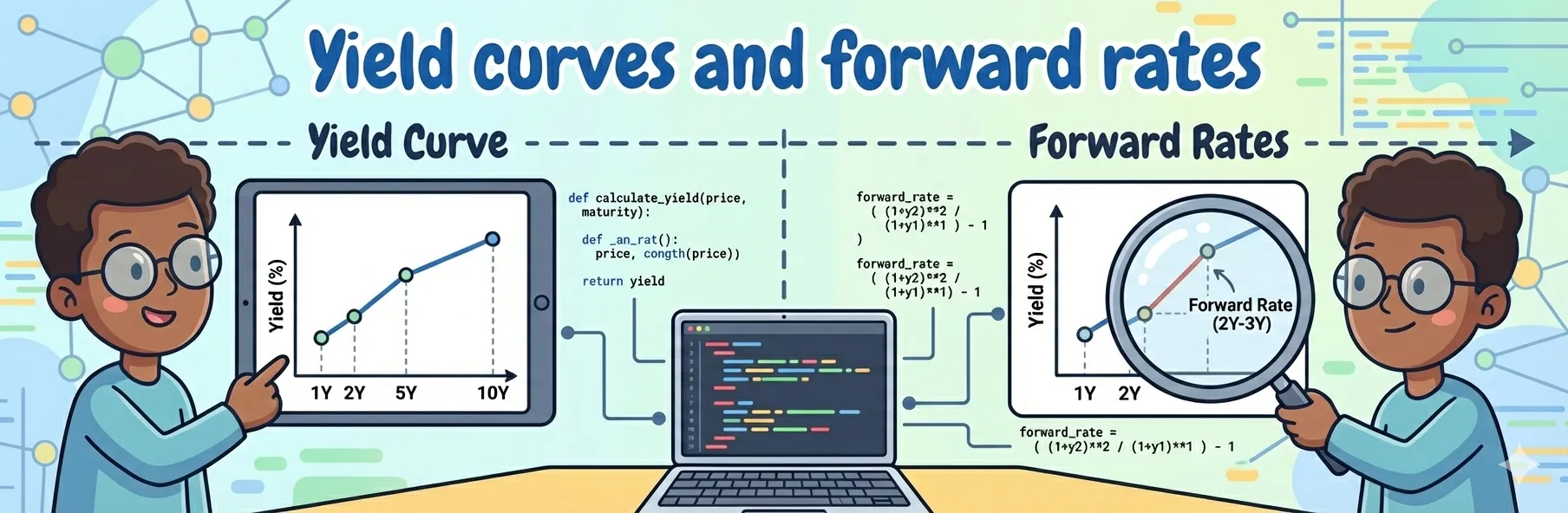
The Geometry of Interest: Constructing Yield Curves and Forward Rates
Master the term structure of interest rates. Learn to build yield curves using bootstrapping and interpolation, and derive forward rates with practical Python examples.
In the world of fixed-income investing, few tools are as misunderstood as yield curves and forward rates. Whether you’re analysing macroeconomic trends, pricing bonds, or assessing interest rate risk, these two concepts are the backbone of modern financial analysis. Despite their importance, many investors struggle to scratch the surface of what they really mean and how to interact with them.
In the previous chapters, we have seen how loans and bonds work, and how we can create more complex financial instruments from them. So far, we have worked with fixed interest rates, but this is not representative of the real world. In more realistic settings, interest rates differ across terms. This variation in interest rate is called the “term structure” of interest rates. With the term structure, we can directly construct the forward rates. The forward rates will help us interpret what the yield means about future interest rates.
In this post, we’ll break down how yield curves work, what forward rates really represent, and why understanding both is essential for interpreting the market’s view of the future. Then we’ll put theory into practice by running simulations, analyzing different curve shapes, and generating visualizations with Python. By the end, you’ll understand these concepts and have hands-on experience exploring them with real data and code.
Constructing Yield Curves
The yield curve is a foundational object in fixed-income markets. It summarizes how interest rates vary with maturity and serves as a critical input for bond pricing, risk management, and the valuation of more complex financial instruments. Despite its importance, the yield curve is not directly observed in the market. Instead, it must be constructed from the prices of traded securities at different points in time. Each of these points on the yield curve represents the interest rate required to exactly reproduce the observed price of a zero-coupon bond () at a given maturity. The price of a zero-coupon bond maturing at time with par value can be written as:
In this notation is the yield corresponding to maturity . It would be easy to construct the yield curve if we had s at every maturity. We would simply observe each price and back out the corresponding yield. In practice, however, this ideal situation does not exist. There are two main challenges:
- Incomplete maturities: Bonds do not mature on every possible date.
- Solution: Estimate missing maturities using interpolation
- Coupon bonds dominate the market: Many traded bonds pay coupons rather than being pure zeros.
- Solution: Synthetically extract prices from coupon bond prices using a procedure known as bootstrapping.
The overall approach to yield curve construction can be summarized as follows:
- Bootstrap zero-coupon prices from observed bond prices for as many maturities as possible.
- Interpolate these zero-coupon prices to obtain values at maturities that are not directly observed.
- Address practical implementation issues, such as market conventions and irregular cash-flow dates.
To understand bootstrapping, it is useful to first ignore interpolation issues and assume that we have sufficient short-dated instruments. The procedure for bootstrapping is:
- Start with Treasury bills (or other short-dated instruments) at the short end of the curve, which are effectively zero-coupon bonds.
- Use the prices of these short-maturity s to compute the present value of coupon payments on longer-dated bonds.
- Subtract the present value of all coupon payments from the observed price of a coupon bond.
- Divide by the principal repayment at maturity to obtain the implied price of a zero-coupon bond for that maturity.
Once we have a collection of prices across maturities, we can invert them to obtain the corresponding yields. This produces the yield curve from short to long maturities.
Using interpolation
Bootstrapping works best when prices are available at many well-spaced maturities. As already mentioned, zero-coupon bonds are rarely issued on every coupon payment date. To make the procedure workable, we must estimate prices at intermediate maturities using interpolation. While many sophisticated interpolation methods exist, for now we will use the basic variant of linear interpolation. Linear interpolation works as follows: Suppose we have observed two points on the curve (, ) and (, ), and wish to estimate the value of at some between and . Linear interpolation gives:
This formula simply traces the straight line connecting the two known data points. Substituting yields and substituting yields . Although it’s a basic form of interpolation, it’s also easy to understand and often sufficient for illustratice purpose. Linear interpolation is also what we will use in our example.
Yield curve example
For our example, we will use the bootstrapping approach. Proceed from short to long maturities using already bootstrapped prices. With the short s, we can turn longer-dated coupon bonds into s. For example:
- A zero-coupon bond with par value and maturity of 6 months has price .
- A coupon bond with par value , annual coupon rate , and maturity of 1 year pays coupons of at 6 months and 1 year, and has a market price .
The price of a synthetic 1-year with par is then obtained by subtracting the present value of the 6-month coupon from the bond price:
The price today of a par maturing at is .
So
So we can get the maturity ** price with an analytic expression. This method works well if you have many prices, well spaced across maturities. We can perform these calculations and construct the yield curve using a Python script.
import numpy as np
import pandas as pd

# Input market data
PAR = 100.0

# Zero-coupon bonds directly observed
# maturity (years) -> price
zcb_prices = {
    0.5: 98.0
}

# Coupon bonds:
# maturity (years), annual coupon rate, market price
coupon_bonds = [
    (1.0, 0.04, 99.0),
    (2.0, 0.05, 101.0),
    (3.0, 0.055, 102.0)
]

# Bootstrapping ZCB prices
def bootstrap_zcb_prices(zcb_prices, coupon_bonds):
    """
    Bootstrap zero-coupon bond prices from coupon bond prices.
    """
    zcb = dict(zcb_prices)  # copy so we can add to it

    for maturity, coupon_rate, price in coupon_bonds:
        coupon = coupon_rate * PAR

        pv_coupons = 0.0
        for t in sorted(zcb.keys()):
            if t < maturity:
                pv_coupons += coupon * zcb[t]

        # Price of synthetic ZCB at maturity
        zcb_price = (price - pv_coupons) / (PAR + coupon)
        zcb[maturity] = zcb_price

    return zcb

zcb_prices = bootstrap_zcb_prices(zcb_prices, coupon_bonds)

# Convert ZCB prices to yields
def zcb_price_to_yield(price, maturity, par=PAR):
    return (par / price) ** (1.0 / maturity) - 1.0

yields = {
    t: zcb_price_to_yield(p, t)
    for t, p in zcb_prices.items()
}

# Linear interpolation
def linear_interpolate(x, x1, y1, x2, y2):
    return y1 + (y2 - y1) * (x - x1) / (x2 - x1)

def interpolate_curve(curve, target_maturities):
    known = sorted(curve.items())
    result = {}

    for x in target_maturities:
        for (x1, y1), (x2, y2) in zip(known[:-1], known[1:]):
            if x1 <= x <= x2:
                result[x] = linear_interpolate(x, x1, y1, x2, y2)
                break

    return result

# Interpolate yields at quarterly maturities
target_maturities = np.arange(0.5, 3.01, 0.25)
interpolated_yields = interpolate_curve(yields, target_maturities)

# Output
df = pd.DataFrame({
    "Maturity (Years)": sorted(interpolated_yields.keys()),
    "Yield": [interpolated_yields[t] for t in sorted(interpolated_yields)]
})

print("Bootstrapped Zero-Coupon Prices:")
for t in sorted(zcb_prices):
    print(f"T={t:.2f}  Price={zcb_prices[t]:.4f}")

print("\nInterpolated Yield Curve:")
print(df.to_string(index=False))The script starts at short maturities with the observed 6-month ZCB. We then bootstrap longer maturities by discounting known coupon payments using previously bootstrapped ZCB prices. Subtracting their present value from the bond price and solving for the implied ZCB price at maturity. With this, we can invert ZCB prices to yields and use interpolation to fill in any missing maturities. From the output of this script, we can see that yields increase with bond maturity.
Finding forward rates
While the yield curve summarizes the cost of borrowing over different maturities as of today, it does not directly tell us how the market prices future borrowing between two dates. Forward rates fill this gap. A forward rate is the interest rate implied by today’s yield curve for a loan that starts at a future date and ends at a later date. So, forward rates translate the information embedded in the yield curve into expectations about the term structure of interest rates over time. In this section, we show how forward rates are derived from zero-coupon bond prices and yields.
It is often known if money will be needed at some time in the future. But this also means we should know what the interest rate will be at that point in the future. For example, somebody may have arranged to buy a new house at time *_in the future and sell an old house at time . They will need the sale of the old house to finance the purchase of the new house. So, at time _,* they can request a bridging loan. The interest on this loan will be the forward rate.
We can infer the forward rate from the yield curve using simple no-arbitrage arguments. The main idea is to investigate over a long horizon where in one step must yield the same return as if we were to take shorter steps of that same horizon. If this is not the case, arbitrage opportunities would exist.
Once more let **denote the price today of a that pays out at maturity . Consider two maturities . A forward rate **is the interest rate, agreed upon today, for a loan that starts at **and matures at time . We can obtain the no arbitrage relationship by combining two strategies.
- Invest directly to :
- Buy a maturing at at price .
- Invest to , then reinvest forward to :
- Buy a maturing at **at price , and at time **reinvest the proceeds at the forward rate .
No arbitrage implies that the value today of both strategies must be equal. This leads to:
Rearranging, the forward rate implied by the yield curve is
Thus, forward rates are fully determined by zero-coupon bond prices. We can write a small python script that takes a bootstrapped yield curve as input to calculate the forward rate.
import numpy as np
import pandas as pd

# Input: spot yield curve
# maturity (years) -> spot rate
spot_rates = {
    0.5: 0.020,
    1.0: 0.025,
    1.5: 0.028,
    2.0: 0.030,
    2.5: 0.032,
    3.0: 0.033
}

# Forward rate calculation
def forward_rate(T1, T2, r1, r2):
    """
    Computes the forward rate f(T1, T2)
    using annual compounding.
    """
    return ((1 + r2) ** T2 / (1 + r1) ** T1) ** (1 / (T2 - T1)) - 1

# Compute consecutive forward rates
maturities = sorted(spot_rates.keys())
forwards = []

for i in range(len(maturities) - 1):
    T1 = maturities[i]
    T2 = maturities[i + 1]
    fwd = forward_rate(T1, T2, spot_rates[T1], spot_rates[T2])
    forwards.append((T1, T2, fwd))

# Output
df = pd.DataFrame(
    forwards,
    columns=["Start (Years)", "End (Years)", "Forward Rate"]
)

print(df.to_string(index=False))
Since prices themselves function as spot zero yields, we can also express forward rates directly in terms of yields. Recall that:
Where *is the spot rate for maturity .* So with this in the script we have substituted into the forward rate formula giving:
Forward rates are implied by current market prices; they are not forecasts in statistical sense. Instead, they represent the rates that make investors indifferent. Under additional assumptions such as risk neutrality we can interpret forward rates as expectations of future spot rates.
Once a smooth yield curve has been constructed via bootstrapping and interpolation, forward rates can be computed for any pair of maturities. This makes forward rates a powerful tool for analyzing the slope and dynamics of the term structure of interest rates.
⚠️ Financial Education Disclaimer
The yield curve construction (bootstrapping) and forward rate models presented here are for educational and analytical purposes only.
- Theoretical Models: These scripts use simplified assumptions (e.g., linear interpolation and annual compounding) that may differ from specific market conventions (like Actual/360 or semi-annual bond equivalent yields).
- No Financial Advice: The outputs of these models do not constitute a recommendation to trade bonds or interest rate derivatives.
- Market Risk: Interest rates are influenced by unpredictable macroeconomic factors, central bank policies, and inflation. Real-world bond pricing includes liquidity premiums and credit spreads not captured in these basic models.
- Code Accuracy: While the logic follows standard financial theory, these scripts should be audited against professional financial libraries (like QuantLib) before being used for actual capital allocation.